Part 1: The Foward Problem

In this exercise, you will implement a solver for the 1D scalar acoustic wave equation with absorbing boundary conditions,

\[\begin{split}(\frac{1}{c(x)^2}\partial_{tt}-\partial_{xx})u(x,t) & = f(x,t), \\ (\frac{1}{c(0)}\partial_t-\partial_x)u(0,t) & = 0, \\ (\frac{1}{c(1)}\partial_t+\partial_x)u(1,t) & = 0, \\ u(x,t) & = 0 \quad\text{for}\quad t \le 0,\end{split}\]

where the middle two equations are the absorbing boundary conditions, the last equation gives initial conditions, \(x \in [0,1]\), and \(t \in [0,T]\). The model velocity is given by the function \(c(x)\).

In our notation, we write that solving this PDE is equivalent to applying a nonlinear operator \(\mathcal{F}\) to a model parameter \(m\), where \(m(x) = \frac{1}{c(x)^2}\) for the scalar acoustics problem.

We then write that \(\mathcal{F}[m] = u\).

Seismic Sources

Before we can solve the equation, we need to define our source function.

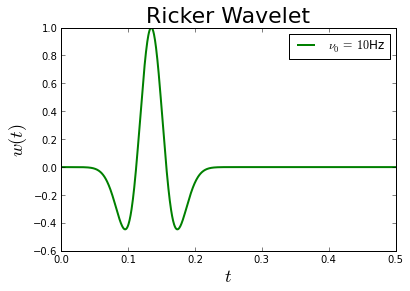
We define our source functions as \(f(x,t) = w(t)\delta(x-x_s)\), where \(\ w\) is the time profile, \(\delta\) indicates that we will use point sources, and the source location is \(x_0\). In real world applications, the time profile is not known and is estimated as part of the inverse problem. However, it is common to model source signals with the negative second derivative of a Gaussian, also known as the Ricker Wavelet,

\[w(t) = (1-2\pi^2\nu_0^2t^2)e^{-\pi^2\nu_0^2t^2},\]

where \(\nu_0\) is known as the characteristic or peak frequency (in Hz), because the magitude of \(w\)’s Fourier transform \(|\hat w|\) attains its maximum at that frequency. It is also important that this function is causal (\(w(t) = 0\) for \(t\le 0\)), so we introduce a time shift \(t_0\),

\[w(t) = (1-2\pi^2\nu_0^2(t-t_0)^2)e^{-\pi^2\nu_0^2(t-t_0)^2}.\]

Problem 1.1

Write a Python function ricker(t, config) which implements the Ricker Wavelet, taking a time t in seconds and your configuration dictionary. This function should assume that your configuration dictionary has a key nu0 representing the peak frequency, in Hz. Your function should returns the value of the wavelet at time t.

You can guarantee causality by setting \(t_0= 6\sigma\) for \(\sigma = \tfrac{1}{\pi\nu_0\sqrt{2}}\), the standard deviation of the underlying Gaussian. You may also want to implement an optional threshold to prevent excessively small numbers.

Plot your function for \(t = 0, \dots, T=0.5\) at \(\nu_0 = 10\textrm{Hz}\) and label the plot.

# In fwi.py

def ricker(t, config):

    nu0 = config['nu0']

    # implementation goes here

    return w

# Configure source wavelet
config['nu0'] = 10 #Hz

# Evaluate wavelet and plot it
ts = np.linspace(0, 0.5, 1000)
ws = ricker(ts, config)

plt.figure()
plt.plot(ts, ws,
         color='green',
         label=r'$\nu_0 =\,{0}$Hz'.format(config['nu0']),
         linewidth=2)
plt.xlabel(r'$t$', fontsize=18)
plt.ylabel(r'$w(t)$', fontsize=18)
plt.title('Ricker Wavelet', fontsize=22)
plt.legend();

Problem 1.2

Write a Python function point_source(value, position, config) which takes a value value, a source location position, and uses the range of the spatial domain config['x_limits'], and the number of points config['nx'] from the configuration to implement a numerical approximation to the \(\delta\). This function should return a numpy array with value at the correct index, correctly evaluating \(w(t)\delta(x-x_s)\) for value = ricker(t). Be careful with your implementation of the numerical delta, as \(\int \delta(x-x_s)\textrm{d}x = 1\).

To implement point_source, we need to discretize the problem domain. This is stored in the configuration as follows:

# Domain parameters
config['x_limits'] = [0.0, 1.0]
config['nx'] = 201
config['dx'] = (config['x_limits'][1] - config['x_limits'][0]) / (config['nx']-1)

For later, we also specify the location of the source:

# Source parameter
config['x_s'] = 0.1

Note

Your function should take a position as a separate parameter and not automatically extract the source location from config because we will re-use this function later.

Wave Solver

The scalar acoustic wave equation can be written as

\[(M\partial_{tt} + A\partial_t + K)u(x,t) = f(x,t),\]

where \(K = K_x + K_{xx}\) is called the stiffness matrix and contains the spatial derivatives, \(A\) is the attenuation matrix and relates to the first time derivatives in the boundary conditions, and \(M\) is the mass matrix and relates to the second time derivatives in the bulk.

Problem 1.3

Write a Python function which construct_matrices(C, config) which constructs the matrices \(M\), \(A\), \(K\) for a given model velocity C. Use a second order accurate finite difference for the second spatial derivative and and use an ‘upwinded’ forward or backward first order difference scheme for the first spatial derivatives.

Hint

It may be helpful to write down precisely what the differential equation looks like at the each interesting point (the two boundaries and some point in the middle of the domain) for your discretized wavefield \(u(j\Delta x, n \Delta t)\).

Hint

The matrices are not time dependent, so \(n\) is fixed. Which \(j\) are relevant at each of the spatial points?

# Load the model
C, C0 = basic_model(config)

# Build an example set of matrices
M, A, K = construct_matrices(C, config)

We can discretize the time derivatives using the usual second-order accurate finite difference approximation,

\[\partial_{tt}u(x,t) \approx \frac{u(x,t-\Delta t) - 2u(x,t) + u(x,t+\Delta t)}{\Delta t^2},\]

which will result in the explicit ‘leap-frog’ scheme for computing \(u(x,t+\Delta t)\). For explicit methods, the stability of the scheme is restricted by the Courant-Friedrichs-Lewy (CFL) condition,

\[\Delta t \le \alpha\frac{\Delta x}{c_\text{max}}.\]

Problem 1.4

Write a Python function leap_frog(C, sources, config) which takes a velocity C, a list of source wavefields sources (one element for each time step), and through the config, takes a time step dt, and a number of time steps nt and returns the time series of wavefields \(u\). Use \(\alpha = \dfrac{1}{6}\) and \(x_s = 0.1\).

Hint

Your leap_frog function should use your construct_matrices function.

# Set CFL safety constant
config['alpha'] = 1.0/6.0

# Define time step parameters
config['T'] = 3  # seconds
config['dt'] = config['alpha'] * config['dx'] / C.max()
config['nt'] = int(config['T']/config['dt'])

# Generate the sources
sources = list()
for i in xrange(config['nt']):
    t = i*config['dt']
    f = point_source(ricker(t, config), config['x_s'], config)
    sources.append(f)

# Generate wavefields
us = leap_frog(C, sources, config)

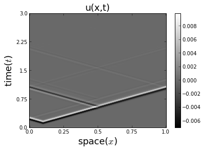
At this point, it is important to visualize the wavefield (and the medium the waves are propagating in). One way to look at the wavefield of a 1D problem is to consider a plot of its space-time diagram.

Problem 1.5

Write a Python function plot_space_time(us, config), using the matplotlib command imshow, to plot and label the space-time diagram for a wavefield \(u(x,t)\).

Hint

The matplotlib xticks and yticks functions will be useful. Try to use a gray-scale color map and consider an optional argument to set the title.

plot_space_time(us, config, title=r'u(x,t)')

Data and Sampling

A receiver (a seismometer, hydrophone, or geophone) at spatial position \(x_r\) records the value of the true wavefield (or a function of it) at a point, and is written mathematically as

\[d_r(t) = d(x_r,t) = \int_\Omega u(x,t) \delta(x - x_r)\textrm{d}x.\]

For 2D and 3D seismic imaging problems there are multiple receivers at different spatial positions recording data for a single ‘shot’ (instance of a source). This ‘sampling’ can be denoted with the operator \(\mathbf{S}\) and is written as

\[\begin{split}\mathbf{d}(t) = \left[ \begin{array}{c} d_{r_1}(t) \\ d_{r_2}(t) \\ \vdots \\ d_{r_n}(t) \end{array} \right] = \left[ \begin{array}{c} \int_\Omega u(x,t) \delta(x - x_{r_1})\textrm{d}x \\ \int_\Omega u(x,t) \delta(x - x_{r_2})\textrm{d}x \\ \vdots \\ \int_\Omega u(x,t) \delta(x - x_{r_n})\textrm{d}x \end{array} \right] = \mathbf{S}u(x,t).\end{split}\]

Your point_source function implements the adjoint operation of sampling, \(\mathbf{S^*}\).

Problem 1.6

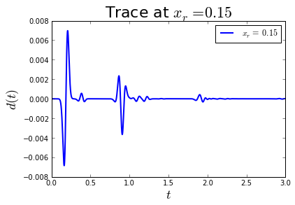
Write a function record_data(u, config), which takes a single wavefield u and, as part of the configuration, a receiver position in config['x_r'] and returns the measured data. When combined, data from all time steps form a trace.

Use \(x_r = 0.15\).

# Receiver position
config['x_r'] = 0.15

Forward Operator

At this point, you have all of the routines necessary to solve the forward problem,

\[\mathcal{F}\left[ m \right] = u.\]

It will be useful to put the necessary steps into a function, as we will want to solve this problem many times, perhaps on different problems. Additionally, we will frequently want to solve the sampled forward problem,

\[\mathbf{S}\mathcal{F}\left[ m \right] = d.\]

Problem 1.7

Write a Python function forward_operator(C, config) which returns a tuple containing the wavefields and the sampled data. This function should utilize the functions you have written in the previous exercises.

Plot and label the trace. Use \(x_r = 0.15\).

Bonus Problems

Bonus Problem 1.8: Derive how you might use your leap_frog function and periodic boundary conditions to design a 4th order accurate, in both space and time, scheme for solving the wave equation.

Bonus Problem 1.9: The implementation of time stepping used in this exercise is not the most efficient approach for implementing time stepping, particularly in higher dimensions. Why? What might be a faster way to implement the time stepping?

Bonus Problem 1.10: The wave equation can be solved using an ODE integrator. Change the formulation of the wave equation so that this is possible. Write a function that uses the built-in SciPy ODE integrator to do your time stepping.