Part 2: The Adjoint State Method

In the previous section, you implemented the nonlinear forward operator

\[\mathcal{F}[m] = u.\]

In the notes, the linearized version of this operator is derived and denoted by the operator \(F\). In this section, you will implement the adjoint of this operator, \(F^*\), and see how the adjoint state method can be used to 1) produce ‘images’ from the imaging condition (Reverse Time Migration) and 2) compute the gradient of the full waveform inversion nonlinear least squares objective function.

The linear forward operator \(F\) is addressed in full in the next section.

Data Residuals

The incident wavefield \(u_0(x,t)\) is generated from the proposal model \(c_0(x)\). The difference between the observed or measured data \(d\) and the simulated data \(d_0\) due to \(u_0\) is called the residual \(r\), and

\[r(t) = d(t) - d_0(t) = d(t) - (\mathbf{S}u)(t) = d(t) - \mathbf{S}\mathcal{F}[m_0] (t).\]

Problem 2.1

Generate the incident field \(u_0\) from the proposal model \(m_0 = \dfrac{1}{c_0^2}\). Compute and plot the residual trace. Be sure to use the same \(\Delta t\) as you did for computing \(u(x,t)\), otherwise you will have to use interpolation to compute the residual.

Adjoint Wave Solver

From the notes, we have that the computed model perturbation \(\delta m\), which we will call the reverse time migration image \(I_\text{RTM}\), is generated by applying the adjoint of the linearized forward model \(F\) to the residual,

\[I_\text{RTM} = F^*r,\]

or, when sampling is taken into account,

\[I_\text{RTM} = (\mathbf{S} F)^*r = F^{*} \mathbf{S}^{*} r = F^*r_{\text{ext}},\]

where \(r_\text{ext}\) is the projection of the residual onto the full wavefield.

Also from the notes,

\[F^*r_{\text{ext}} = -\int_0^T q(x,t) \partial_{tt}u_0(x,t) \textrm{d}t,\]

where \(q(x,t)\) is the solution of

\[\begin{split}(\frac{1}{c_0(x)^2}\partial_{tt}-\partial_{xx})^{*}q_t(x,t) & = r_\text{ext}(x,t), \\ (\frac{1}{c_0(0)}\partial_t-\partial_x)^{*}q(0,t) & = 0, \\ (\frac{1}{c_0(1)}\partial_t+\partial_x)^{*}q(1,t) & = 0, \\ u(x,t) & = 0 \quad\text{for}\quad t \ge T,\end{split}\]

where the adjoint operation \(*\) is taken in time and collectively \(L_0^{*}q(x,t) = r_\text{ext}(x,t)\) (as opposed to \(Lu(x,t)=f(x,t)\) for the true wavefield). (Note that the argument \(r_\text{ext}\) can be replaced by any wavefield, \(F*\) is defined for any argument, not just the extended residual.)

Problem 2.2

Extend your residual to the whole space using your point_source function at the receiver location \(x_r\), to create a list of adjoint source wavefields . Using your leap_frog function, solve for the adjoint field \(q(x,t)\). Plot the space-time diagram of \(q(x,t)\).

Hint

Be very careful, as the absorbing boundary conditions imply that \(L\ne L^*\). What does the adjoint operation mean in the time domain? How does this impact the time derivatives and your discretization of those derivatives?

Imaging Condition

As mentioned before, the perturbation is

\[I_\text{RTM} = F^*\mathbf{S}^*r = \int_0^T\ q(x,t) \partial_{tt}u_0(x,t) \textrm{d}t,\]

this inner product is known as an imaging condition and is the core of a gradient based optimization method. The image \(I_\text{RTM}\) is said to have been produced by Reverse Time Migration.

Problem 2.3

Write a Python function imaging_condition(qs, u0s, config) that computes \(F^*r_\text{ext}\), given the incident wavefield \(u_0\).

You may want to write a separate function to compute the second time derivative of the incident field. You can assume that \(u_0 = 0\) for \(t > T\).

Hint

Don’t forget to account for the measure in your integrals.

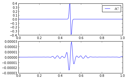
Plot the resulting image of the reflection. Compare that image to \(\delta C = C - C_0\). Think about how and why they are different? How might these results change if the source and receiver are on opposite sides of the reflector? What if there are multiple receivers?

# Compute the image
I_rtm = imaging_condition(qs, u0s, config)

# Plot the comparison
xs = np.arange(config['nx'])*config['dx']
dC = C-C0

plt.figure()
plt.subplot(2, 1, 1)
plt.plot(xs, dC, label=r'$\delta C$')
plt.legend()
plt.subplot(2, 1, 2)
plt.plot(xs, I_rtm, label=r'$I_\text{RTM}$')
plt.legend()

Visualizing the imaging condition as a space-time diagram is a very good way to understand how the intersection of the incident and adjoint waves locates the reflectors.

Problem 2.4

Visualizing the imaging condition. Plot the space-time diagram for \(\partial_{tt}u_0(x,t)\). Either print the space-time diagrams of \(q(x,t)\) and \(\partial_{tt}u_0(x,t)\) and overlay them or use matplotlib to overlay the two images. See where the adjoint field and the incident field intersect to find the location of the reflection. Try to understand why the intersections appear where they do.

Adjoint Operator

The adjoint operator is a linear operator and it will be useful to have a way to apply it as a black box, much like we have a function forward_operator for applying the nonlinear forward operator as a black box.

Problem 2.5

Write a function adjoint_operator(C0, d, config) which implements the adjoint operation you developed in Problems 2.2 and 2.3 and returns the reverse time migration image. Consider optionally returning the adjoint field.

Hint

Remember that the argument d can be anything that ‘looks like’ data. For example, the residual.