Note
The problem in this example is small enough that it can be run in serial on a normal laptop in (at worst) a few minutes. For a more complex example that should run in parallel, see 2D Marmousi Velocity Model.
This example is a quick guide to the general structure of a PySIT seismic
inversion script. You can either type the commands into the IPython console,
or you can copy sections in by copying the text and using the %paste
IPython magic function.
2D Horizontal Reflectors
The source code for a slightly more complex version of this example is found in the
PySIT examples directory: examples/HorizontalReflector2D.py.
Set Up the Computing Environment
To get started, start an IPython console with the command
ipython --pylab
First, we must import some fairly standard python and numerical python libraries that we will use in this demo. Run the following commands:
import numpy as np
import matplotlib.pyplot as plt
to import the numpy module, which contains the basic numerical array functionality (we have chosen to abbreviate it with the standard shorthand np), and the matplotlib plotting library which we also abbreviate as is the standard.
Next, import all of the basic functionality of the pysit module:
from pysit import *
This will give access to almost everything we need. However, the gallery examples are not imported with the previous statement, so we must import the horizontal_reflector module separately:
from pysit.gallery import horizontal_reflector
Set Up the Model Problem
PySIT is designed to model the physical observation geometry in as intuitively as possible. Generally the first thing that needs to be done is to define a physical and computational domain in which to work:
pmlx = PML(0.1, 100)
pmlz = PML(0.1, 100)

x_config = (0.1, 1.0, pmlx, pmlx)
z_config = (0.1, 0.8, pmlz, pmlz)
These lines define the x and z boundaries of the domain in physical coordinates (arbitrary units for this example) and the boundary conditions on the left and right sides of each dimension. PySIT works in the typical left handed coordinate system of geophysics (Z points down).
Currently, the PySIT supports Dirichlet boundaries and absorbing boundaries
implemented using a perfectly matched layer (PML), which is defined using the PML
class. The PML is specified in the same physical units as the
domain. Here, we have defined the PML to have length 1/10 units, in each
direction, with a PML intensity parameter of 100. Finally, we can define the
domain itself:
domain = RectangularDomain(x_config, z_config)
PySIT works for 1D, 2D, and 3D problems. We have chosen a 2D example. The argument list to the domain constructor is a configuration tuple for each dimension. The constructor uses the number of these configurations to determine the dimension of the problem. Most procedural gallery problems require you to create a physical domain, most community/precomputed gallery problems generate domains and meshes for you.
After the physical domain is specified, we must specify a computational domain or a mesh:
mesh = CartesianMesh(d, 91, 71)
The Cartesian mesh takes a domain as its first parameter, and then the number of grid points in each dimension as the remaining arguments. Note that both end points are included, so this will ensure that the grid spacing is 0.01.
Finally, create the reflection model:
C, C0, mesh, domain = horizontal_reflector(mesh)
Note
horizontal_reflector is a convenience function for generating problem
setups. All of these convenience functions have the same return
signature, a tuple containing:
- the true model,
- an initial model,
- the computational mesh,
- the computational domain.
This means that, occasionally, some variables are passed in and returned by the function. Some gallery examples (e.g., Marmousi) generate the domain and mesh as well, but we must create one to use the horizontal reflector gallery model.
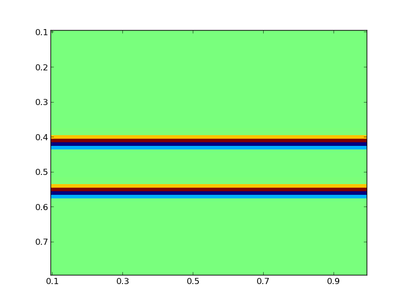
Here, we have acoustic model parameters defined such that C^-2 = C0^-2 + dM. Thus, C is the true wave speed, C0 is the initial non-oscillatory model, and dM, which is not returned, is the perturbation of the model. The model problem can be plotted by:
plt.figure()
vis.plot(C, mesh)
plt.draw()
The plot command used is part of the visualization tools provided by PySIT. The result should be a figure that looks like this:
Set Up the Sources and Receivers
For this example, we will use a single shot. A shot is a source coupled with a receiver or a group of receivers. Before going on, let us extract some useful information:
zmin = d.z.lbound
zmax = d.z.rbound
zpos = zmin + (1./9.)*zmax
zmin and zmax are the left and right (or top and bottom) physical boundaries of the domain. Alternatively, we could hard code these from the specification above, but this is a good time to introduce a useful property of the domain: The spatial properties of the domain are typically described without the boundary/ghost conditions.
In this example, d.z.lbound (the top physical coordinate) has the value 0.1 and d.z.lbc.length (the physical size of the top PML) has the value 0.1. Thus, the effective domain has a top boundary of 0.0 when boundary conditions are included. The boundary conditions only come into play during the wave propagation phases.
For testing, a common acquisition regime is the equispaced acquisition, where
sources and receivers are even spaced across the domain at a fixed depth.
PySIT provides a convenience routine for creating one
(equispaced_acquisition):
shots = equispaced_acquisition(mesh,
                               RickerWavelet(10.0),
                               sources=1,
                               source_depth=zpos,
                               receivers='max',
                               receiver_depth=zpos)
For this case, we have chosen one to use one source, at the previous specified
depth (which is the ‘top’ of the domain and not in the PML region) and the
maximum number of receivers (the number of horizontal grid points) at the same
depth. Because we chose equispaced sources, the single source is in the middle
of the domain. The source function itself is a Ricker wavelet with peak
frequency of 10Hz. The return value, shots is a list of Shot objects.
Each Shot object contains a source-receiver pair (or a
PointSource-ReceiverSet pair, to be more specific). The portions of PySIT
that deal with shots, expect collections of shots to be in a Python list.
Define the Solver and Generate Synthetic Data
PySIT defines solvers as objects that are passed to different routines. This
is so that all code that uses wave solvers remains generic. Any PySIT solver
object can be used here, but we will use a solver for the constant-density
acoustic wave equation, ConstantDensityAcousticWave. The factory for
ConstantDensityAcousticWave automatically determines the correct dimension
for the solver based on the mesh that is provided.
solver = ConstantDensityAcousticWave(mesh,
                                     formulation='scalar',
                                     spatial_accuracy_order=2,
                                     trange=(0.0, 3.0),
                                     kernel_implementation='cpp')
The first argument is, again, the mesh, the second specifies that we are using the scalar form of the equation, and the third specifies the set of wave parameters that are to be used in the solve. Finally, we specify the time range (in seconds), the spatial accuracy, and to use an accelerated solver.
This solver is then used to generate some seismic data:
wavefields = []
base_model = solver.ModelParameters(mesh, {'C': C})
generate_seismic_data(shots,
                      solver,
                      base_model,
                      wavefields=wavefields)
We pass the list of shots and the solver we chose to the data generation
routine. The first line generates an empty list that will be passed as an
argument to the data generation routine. This tells the routine to extract the
wave evolution in the list wavefields, which can be viewed with the
PySIT animation function vis.animate:
vis.animate(wavefields, mesh, display_rate=10)
After the routine has run, each receiver will have its trace stored internally.
Objective Function and Solving the Inverse Problem
To solve an inversion problem in PySIT, you must specify an objective function and an algorithm for optimizing it. PySIT currently defines the least-squares objective in the time and frequency domains, as well as a hybrid approach. Objective functions require wave equation modeling, and thus are dependent upon our solver. Here, we define the time-domain objective:
objective = TemporalLeastSquares(solver)
PySIT defines inversion methods as stateful objects. Currently, PySIT supports gradient descent, L-BFGS, and more. L-BFGS is the preferred method:
invalg = LBFGS(objective)
The inversion algorithm requires the objective function of choice to be specified as an argument. Additionally, we need an initial value, so define that as well:
initial_value = solver.ModelParameters(mesh, {'C': C0})
Next, we must configure the optimization routine’s diagnostic recording. Each of the following dictionary entries specify the frequency (in iterations) with which the listed value is stored:
status_configuration = {'value_frequency': 1,
                        'residual_frequency': 1,
                        'residual_length_frequency': 1,
                        'objective_frequency': 1,
                        'step_frequency': 1,
                        'step_length_frequency': 1,
                        'gradient_frequency': 1,
                        'gradient_length_frequency': 1,
                        'run_time_frequency': 1,
                        'alpha_frequency': 1}
Finally, we can run the optimization routine:
nsteps = 15
result = invalg(shots,
                initial_value,
                nsteps,
                line_search='backtrack',
                status_configuration=status_configuration,
                verbose=True)
This will run 15 iterations of L-BFGS starting from initial_guess using a backtracking line search. There are other optional arguments (that can be seen in the documentation) that allow for extraction of intermediate values and tracking of things like the residual history.
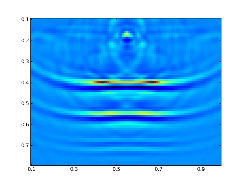
Finally, we can plot the resulting model:
plt.figure()
vis.plot(result.C, m)
plt.draw()
Where you should see a figure that looks like this:
Additionally, you can look at the descent behavior of the algorithm by plotting the objective values:
obj_vals = np.array([v for k,v in invalg.objective_history.items()])
plt.figure()
plt.semilogy(obj_vals)
Or you can look compare the true, initial, and final solutions:
clim = C.min(),C.max()
plt.figure()
plt.subplot(3,1,1)
vis.plot(C0, m, clim=clim)
plt.title('Initial Model')
plt.subplot(3,1,2)
vis.plot(C, m, clim=clim)
plt.title('True Model')
plt.subplot(3,1,3)
vis.plot(result.C, m, clim=clim)
plt.title('Reconstruction')
plt.draw()