Warning

The problem in this example is designed to be run in parallel. It can be run in serial, but it will be very expensive. It is strongly recommended that you go through the simpler example above, first.

2D Marmousi Velocity Model

The source code for this example is in the PySIT examples directory or can be downloaded here: ParallelMarmousi.py.

Set Up the Computing Environment

Unlike the previous example, this demo uses parallelism with MPI. It is possible to use MPI together with IPython, but we will use this example to introduce a way to save and load computed images.

Running the Script

The following command runs the script in parallel over <nprocs> processors:

mpirun -n <nprocs> python ParallelMarmousi.py

Details of ParallelMarmousi.py

Setup the standard import block. The time standard library module provides access to date, time, and timing routines. The sys standard library module provides access to many things, in this case we will use it to write to stdout.

import time
import sys

import numpy as np

Here we import the necessary PySIT tools. In particular, we are importing the function interface to the pysit.gallery.marmousi community gallery problem. Additionally, we import the ParallelWrapShot class to tell PySIT how to handle parallelism over shots.

from pysit import *
from pysit.gallery import marmousi

from pysit.util.parallel import ParallelWrapShot

Of course, we will also need access to MPI routines.

from mpi4py import MPI

The block if __name__ == '__main__': is a way to tell the Python interpreter not to execute this code if the file is simply imported. Here, we are executing the script, so anytyhing inside this block will be executed.

For convenience, we create local references to some relevant MPI properties.

if __name__ == '__main__':

    comm = MPI.COMM_WORLD
    size = comm.Get_size()
    rank = comm.Get_rank()

This line constructs a wrapper on the COMM_WORLD MPI communicator and essentially tells PySIT that shots will be distributed evenly over the processors.

    # Wrapper for handling parallelism over shots
    pwrap = ParallelWrapShot(comm=MPI.COMM_WORLD)

Construct the true velocity, initial velocity, computational mesh, and physical domain for a small patch of the Marmousi velocity model. The patch keyword tells marmousi() that we will use a small, predefined section of the full velocity model.

Warning

If a patch of a community gallery model, at a particular resolution, has not been used before, PySIT will generate it and store it. There currently exists a race condition that can cause issues if a script is running in parallel and the patch has not been precomputed. It is recommended that you precompute this patch by:

1. Opening an IPython console
2. Running from pysit.gallery import marmousi
3. Running C, C0, m, d = marmousi(patch='mini_square')

This needs to be done only once.

    #   Load or generate true wave speed
    C, C0, m, d = marmousi(patch='mini_square')

For this problem, we are using one shot per processor, so the size of the communicator defines the number of shots for the problem. Note that the call to equispaced_acquisition() takes a keyword for the parallel wrapper. This allows the acquisition function to evenly distribute construction of the list of shots. The returned list of shots will contain only the shots assigned to the current processor.

    Nshots = size
    sys.stdout.write("{0}: {1}\n".format(rank, Nshots // size))

    shots = equispaced_acquisition(m,
                                   RickerWavelet(10.0),
                                   sources=Nshots,
                                   source_depth=20.0,
                                   receivers='max',
                                   parallel_shot_wrap=pwrap,
                                   )

As before, define the wave solver.

    trange = (0.0,3.0)

    solver = ConstantDensityAcousticWave(m,
                                         spatial_accuracy_order=6,
                                         trange=trange,
                                         kernel_implementation='cpp')

And generate the data. Note that the parallel wrapper is not needed here, as each shot exists only on the processor that owns it and each piece of data can be generated independently.

    base_model = solver.ModelParameters(m,{'C': C})
    tt = time.time()
    generate_seismic_data(shots, solver, base_model)
    data_gen_time = time.time()-tt

An MPI Barrier allows the processors to synchronize after generating the data.

    comm.Barrier()

Define the objective function. As the objective function contains an explicit summation over shots, we must pass the parallel wrapper to the constructor so that the summation can occur when the objective is evaluated and gradients are computed.

    objective = TemporalLeastSquares(solver,
                                     parallel_wrap_shot=pwrap)

Define the optimization routine and set the initial value to be the velocity that we generated with the gallery problem.

    # Define the inversion algorithm
    invalg = LBFGS(objective, memory_length=10)

    initial_value = solver.ModelParameters(m, {'C': C0})

Configure and run the optimization for 10 steps, storing the reconstructed model and the value of the objective function at every iteration.

    nsteps = 10

    status_configuration = {'value_frequency'           : 1,
                            'objective_frequency'       : 1}

    result = invalg(shots, initial_value, nsteps,
                    line_search='backtrack',
                    status_configuration=status_configuration,
                    verbose=True)

Finally, only one processor needs to save the data. The SciPy io function savemat() will save a dictionary of numpy arrays in the MATLAB file format. Here, we save the reconstruction, the true model, the initial mode, and an array of the objective values to a file called marm_recon.mat.

    if rank == 0:

        model = result.C.reshape(m.shape(as_grid=True))

        vals = list()
        for k,v in list(invalg.objective_history.items()):
            vals.append(v)
        obj_vals = np.array(vals)

        from scipy.io import savemat

        out = {'result': model,
               'true': C.reshape(m.shape(as_grid=True)),
               'initial': C0.reshape(m.shape(as_grid=True)),
               'obj': obj_vals
              }
        savemat('marm_recon.mat',out)

On 12 cores of a 16 core Intel Xeon E5-2670 machine, this script runs in roughly 25 minutes.

Visualizing the Results

Start an IPython console with the command

ipython --pylab

Then, import the SciPy function loadmat().

from scipy.io import loadmat

Next, load the .mat file the script created.

result = loadmat('marm_recon.mat')

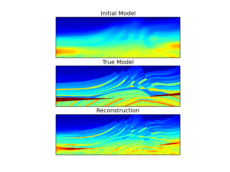
Now we can plot the three models on the same color scale.

clim = result['true'].min(), result['true'].max()

plt.figure()

plt.subplot(3,1,1)
plt.imshow(result['initial'].T, clim=clim)
plt.title('Initial Model')
plt.xticks([])
plt.yticks([])

plt.subplot(3,1,2)
plt.imshow(result['true'].T, clim=clim)
plt.title('True Model')
plt.xticks([])
plt.yticks([])

plt.subplot(3,1,3)
plt.imshow(result['result'].T, clim=clim)
plt.title('Reconstruction')
plt.xticks([])
plt.yticks([])

Finally, we can plot the behavior of the objective function.

plt.figure()
plt.semilogy(result['obj'][0])